Microwave grouper

The processes of beam bunching in a microwave buncher can be analyzed using the equations of longitudinal dynamics:

Equation for the change in particle momentum

\[\frac{dp_z}{dt} = eE(z)\cos(\omega t + \phi_0)\]

where \(p_z\) is the longitudinal momentum of the particle, \(e\) is the charge of the electron, \(E(z)\) is the distribution of the magnitude of the longitudinal electric field along the axis of the buncher, \(\omega\) is the angular frequency, and \(\phi_0\) is the initial phase. Taking into account that the longitudinal momentum of a particle is \(\beta\gamma m\), where \(m\) is the rest mass of an electron, and \(\beta\) and \(\gamma\) are the usual relativistic factors of particles, equation can be rewritten as

Equation for the change in longitudinal phase space

\[\frac{d(\gamma\beta)}{dt} = \left(\frac{e}{mc}\right)E(z)\cos(\omega t + \phi_0)\]

The derivative $:nbsphinx-math:frac{dgamma beta}{dt} = \dot{\gamma}\beta `+ :nbsphinx-math:dot{beta}`:nbsphinx-math:`gamma `$, where the dot indicates a derivative with respect to time, can be transformed as follows:

\[\dot{\gamma} = \frac{d}{dt} \frac{1}{\sqrt{1-\beta^2}} = \beta \gamma^3 \dot{\beta}.\]

Then takes the form:

\[\frac{d\gamma \beta}{dt} = \gamma \dot{\beta} (\gamma^2 \beta^2 + 1) = \frac{e}{mc} E(z) \cos(\omega t + \varphi_0).\]

If we assume that the longitudinal velocity of the particle is much smaller than the transverse velocity \(\gamma \beta_{\alpha, r} \ll \gamma \beta\), then \(\gamma^2 = \gamma^2 \beta^2 + 1\), and transitioning to the longitudinal coordinate \(dt = \frac{dz}{\beta c}\), we get:

\[\frac{d\beta}{dz} \frac{\beta }{(1-\beta^2)^{3/2}} = \frac{E(z)}{U_0} \cos(\varphi + \varphi_0),\]

where \(U_0 = mc^2/e\) - is the rest energy of the electron in volts, \(\varphi\) - is the phase of the moving particle relative to the electrical component of the CBM field:

\[\frac{d\varphi}{dz} = \frac{\omega}{\beta c}.\]

import numpy as np
import matplotlib.pyplot as plt

# Constants
U0 = 511e3  # Rest energy of the electron in eV (mc^2/e)
c = 3e8  # Speed of light in vacuum (m/s)
omega = 2 * np.pi * 1e9  # Angular frequency (for example, 1 GHz)
f = 1.5 * 1e9  # Frequency
phi_0 = 0  # Initial phase
E0 = -40e6  # Electric field strength in V/m (example value)
dz = 1e-5  # Step size in m
z_max = 0.9  # Length of the buncher in m
z_max_grouper = 0.3  # Length of the buncher in m
num_particles = 1_000  # Number of particles

# Initial conditions
betas = np.full(num_particles, 0.7)  # Initial beta for all particles
phis = np.linspace(0, np.pi, num_particles)  # Uniform distribution of initial phases

# Function to calculate derivatives
def derivatives(beta, phi, E):
    dbeta_dz = (E / U0) * np.cos(phi + phi_0) * ((1 - beta**2)**(3/2)) / beta
    dphi_dz = omega / (beta * c)
    return dbeta_dz, dphi_dz

# Function to calculate Ez(z)
def E_z(z):
    return np.where(z < z_max_grouper, E0 * np.sin(2 * np.pi * f * z / c + phi_0), 0)

# Solving the system using Euler's method
z_values = np.arange(0, z_max, dz)
betas_values = []
phis_values = []

for z in z_values:
    dbeta_dz, dphi_dz = derivatives(betas, phis, E_z(z))
    betas += dbeta_dz * dz
    phis += dphi_dz * dz
    betas_values.append(betas.copy())
    phis_values.append(phis.copy())

# Correcting phase to be within [0, 2*pi]
phis = phis % (2 * np.pi)

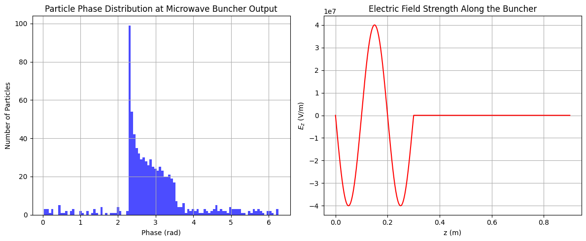
# Plotting the histogram of particle phases at the output
plt.figure(figsize=(12, 5))
plt.subplot(1, 2, 1)
plt.hist(phis, bins=100, color='blue', alpha=0.7)
plt.xlabel('Phase (rad)')
plt.ylabel('Number of Particles')
plt.title('Particle Phase Distribution at Microwave Buncher Output')
plt.grid(True)

# Plotting Ez(z)
Ez_values = E_z(z_values)
plt.subplot(1, 2, 2)
plt.plot(z_values, Ez_values, label='$E_z(z)$', color='red')
plt.xlabel('z (m)')
plt.ylabel('$E_z$ (V/m)')
plt.title('Electric Field Strength Along the Buncher')
plt.grid(True)
plt.tight_layout()
plt.show()

D:\TMP\ipykernel_8688\75803242.py:22: RuntimeWarning: invalid value encountered in power
  dbeta_dz = (E / U0) * np.cos(phi + phi_0) * ((1 - beta**2)**(3/2)) / beta